$AGILE_DIR/tests/{hd,mhd,ffhd,srhd}/ holds AGILE's test suite: a mix of short regression cases (built and run automatically by make hd/make mhd/make ffhd, see Getting Started) and larger, physically motivated setups used as science demonstrations. This page documents the examples that are also described in detail in the AGILE 1.0 paper, Porth et al., "Astrophysics on GPUs: introducing AGILE 1.0" (submitted to RASTI, in review; arXiv:2607.19277) -- the citable reference for AGILE 1.0 (see also Acknowledgments). Section numbers below refer to that paper. To run any of them yourself, build and launch it the same way as in Getting Started, e.g.

cd $AGILE_DIR/tests/hd/KH3D
make arch=gnu
mpirun -np 4 ./agile -i agile.par

Beyond the examples below, tests/ contains further regression and verification setups (e.g. hd/RT3D, hd/KH3D-SMR, hd/KH3D_tracer, hd/sphere_advection, mhd/blast_wave_Cartesian_3D, mhd/Orszag-Tang_3D, mhd/doubleGEM3D, srhd/shockTube) that aren't individually described in the paper and so aren't covered here.

Hydrodynamics (tests/hd/)

Double Kelvin-Helmholtz benchmark -- KH3D

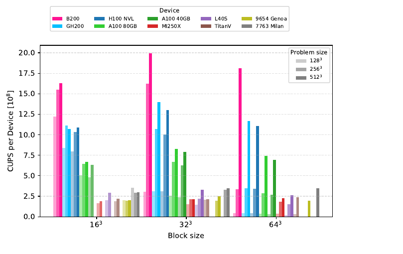
(paper Sections 3.1-3.2) Used to establish AGILE's baseline single- and multi-GPU performance, rather than as a physics validation case. A fully periodic, uniform-grid 3D domain [0,1]^3 is set up with a horizontal velocity field that switches sign twice across the domain height, so the flow is Kelvin-Helmholtz unstable at two shear layers at once (hence "double" Kelvin-Helmholtz). It uses Lax-Friedrichs (tvdlf) fluxes, van Leer slope limiting and a three-step Runge-Kutta update; the code is advanced for 100 timesteps and the average cell updates per second (CUPS) is recorded. The paper's Figure 5 and Table 2 report measured performance across device types (up to ~2x10^9 CUPS on an NVIDIA B200), and Section 3.2 reports multi-GPU strong- and weak-scaling results up to 2048 GPUs on the Snellius and LUMI-G clusters.

Double Mach reflection meets shock-cloud -- Woodward_Collela

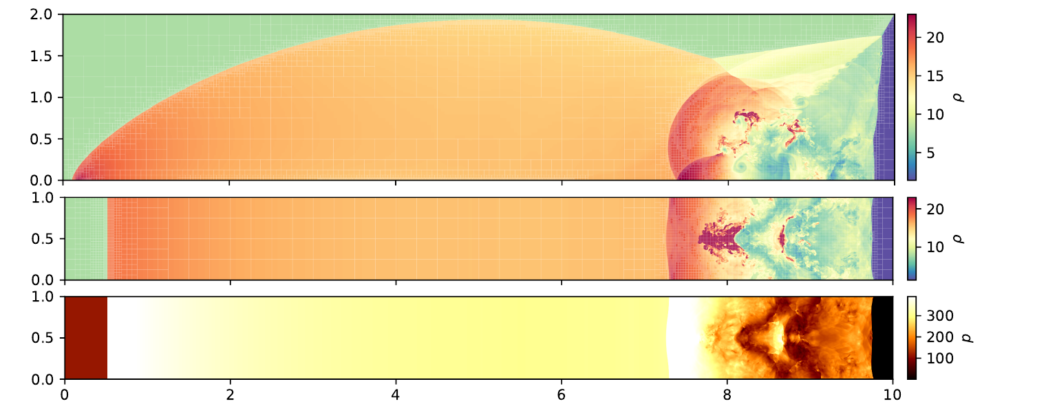
(paper Section 4.1) Combines the classic Mach-10 double-Mach-reflection shock test of Woodward & Colella (1984) with a dense spherical cloud embedded in the pre-shock flow, demonstrating the hydrodynamics module together with shock-capturing and adaptive mesh refinement in a genuinely 3D setting. The initial condition sets three uniform states in contact: a static pre-shock medium (density ρ = γ̂ = 1.4, pressure p = 1), a static spherical cloud of density ρ = 10 and radius 0.25 centered at (x,y,z) = (7,0,0.5) in pressure equilibrium with the pre-shock gas, and a moving Mach-10 post-shock state (ρ = 8, p = 116.5, shock-normal velocity 8.25) separated by a planar shock front angled at 60° to the x-axis. The domain is (Lx,Ly,Lz) = (10,2,1), with reflective walls at z=0,1, continuous outflow at x=10, and time-dependent boundary states at x=0 and y=2 that track the moving Mach-10 shock. HLLC fluxes, van Leer reconstruction and a three-step Runge-Kutta update are used, evolved to t=0.9. As the shocked cloud interacts with the reflection pattern it develops Richtmeyer-Meshkov deformations and further Kelvin-Helmholtz roll-ups.

agile.par runs a lighter refine_max_level=3 version of this setup for local testing; agile_wc3d_6l_big.par (paired with the job_lumi_gpu_6l*.sh batch scripts) reproduces the paper's full 6-level production run at effective resolution 7680×1536×768, which at peak activated over a million AMR blocks (1.7×10^9 cells) and ran for 2944 node-hours across up to 2048 GPUs on LUMI. This case is a science demonstration, not part of the automated make hd regression suite.

Multiphase turbulent mixing -- TRML

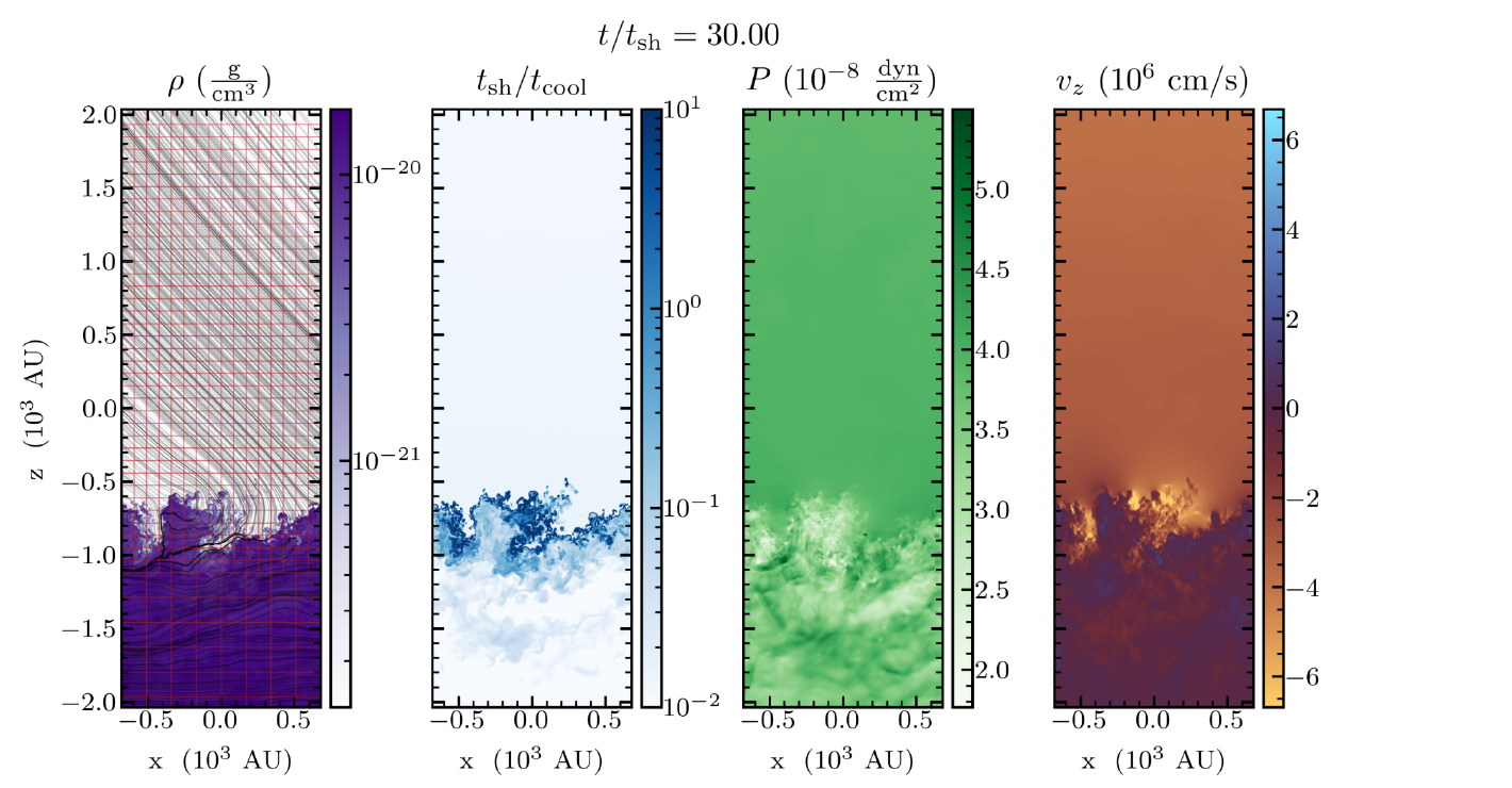
(paper Section 4.2) A 3D turbulent radiative mixing layer (TRML) forming between a hot, tenuous phase and a cold, dense phase in shear contact -- relevant to interfaces between hot coronal/circumgalactic gas and cooler clouds. The Kelvin-Helmholtz-unstable shear setup follows the 2D noisy benchmark of Lecoanet et al. (2015), generalized to 3D with band-limited white noise at the interface; the radiative mixing layer physics follows Fielding et al. (2020), using a hand-crafted log-skew-normal cooling curve Λ(T) (mixing temperature T = 0.2 MK, cold-phase density ρc = 10^-20 g/cm^3, peak Λ(T) = 8×10^-22 g cm^5/s^3) chosen so the cold and hot phases radiate comparably. The temperature/density contrast between phases is χ = 100, the ratio of the shear to cooling timescale is ξ = 10, and the hot phase is mildly subsonic (Mach 0.3) while the cold phase is supersonic. HLLC fluxes, van Leer reconstruction and a three-step Runge-Kutta update are used, with custom static mesh refinement concentrated on the mixing layer.

A thin, fractal mixing layer develops as the layer migrates upward, absorbing hot-phase material; the paper quantifies its fractal dimension by subsampling AMR blocks (or isosurfacing) on a cooling-to-shear timescale ratio, measuring d = 2.541, consistent with the d = 5/2 scaling predicted by Fielding et al. (2020). Performance on LUMI reached ≳1.5×10^8 CUPS per GCD, close to AGILE's uniform-grid single-GPU benchmark number.

Cloud crushing -- cloud_crushing

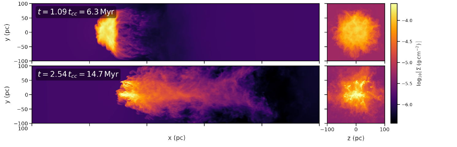
(paper Section 4.3) The classic "cloud crushing" problem (Klein et al. 1994): a cold, dense cloud is struck and disrupted by a hot wind, following the setup of Girichidis et al. (2021). A wind of temperature Tw = 10^6 K, number density nw = 10^-3 cm^-3 and velocity vw = 100 km/s enters continuously from the domain's left boundary; a spherical cloud of radius rc = 50 pc sits in pressure equilibrium with the wind at one of three density contrasts χ = ρc/ρw ∈ {140, 240, 340}. The wind drives a Mach ≈ 10 shock into the cloud, triggering Kelvin-Helmholtz and Rayleigh-Taylor instabilities at the cloud-wind interface that ablate and mix cloud material downstream; a seeded turbulent velocity field (Burgers spectrum, vrms = 1 km/s) and small density asymmetry break symmetry to promote realistic mixing. Radiative cooling uses the Colgan_DM curve (Colgan et al. 2008 at high temperature, Dalgarno & McCray 1972 at low temperature). The domain spans 20rc × 4rc × 4rc with the cloud centered at x = 5rc.

The paper's default (χ = 240) run uses MUSCL reconstruction with a van Leer limiter, the HLLC solver and three-step Runge-Kutta time integration, on a base grid of 320×64×64 with 3 AMR levels (block size 32^3, up to 4096 blocks; effective resolution 1280×256×256), refined with Löhner's indicator on a weighted combination of the passive tracer (80%) and density (20%). Diagnostics track the cloud velocity v25(t) (the velocity at the 25th percentile of the mass distribution along x) against the analytic ram-pressure drag prediction, and the cold cloud mass fraction fcl(t); fitted drag coefficients CD ≈ 3.1 are consistent across all three density contrasts. Uniform-grid performance runs (1280×256×256, HLL solver, 32 MI250X GCDs on LUMI) reached ~1.1×10^8 CUPS/GCD.

Frozen-field hydrodynamics (tests/ffhd/)

Multiphase dynamics in the solar corona -- quadrupolar3D

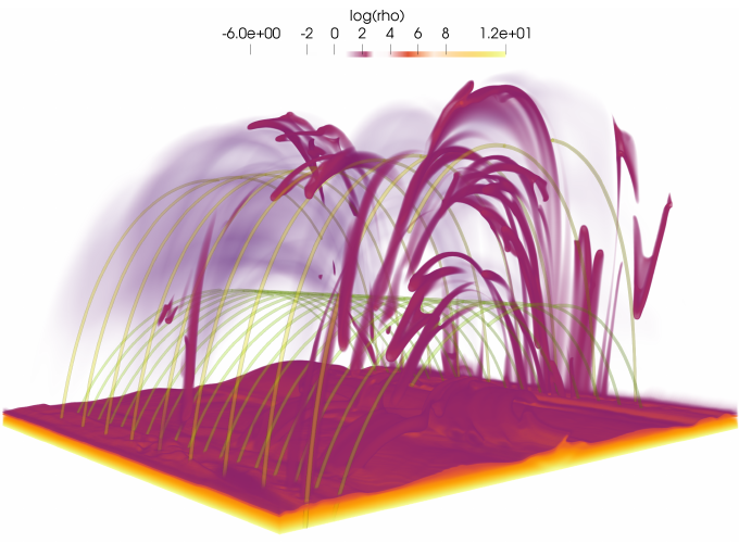
(paper Section 4.4) Demonstrates the 3D frozen-field hydrodynamics (FFHD) module -- a field-aligned hydrodynamic module (see paper Section 2.3.2) that solves mass, momentum and energy transport along a static, prescribed 3D magnetic field, including anisotropic (field-aligned) thermal conduction. The magnetic topology is a quadrupolar two-arcade structure (a fundamental arcade superposed with a third-harmonic arcade) with a shear component that decreases with height, following the evaporation-condensation prominence models of Xia et al. (2012) and Keppens & Xia (2014) but generalized from their 2.5D configuration into a genuinely 3D sheared-loop system. The domain is [-5,5]x[-5,5]x[0,5] in units of 10 Mm, resolved by a uniform 600^3 grid (83.3 km resolution), initialized as a gravitationally stratified chromosphere-transition-region-corona atmosphere with Colgan_DM radiative losses. The atmosphere is first relaxed under a background volumetric heating term, then a localized, stochastic heating term (following Zhou et al. 2020 and Li et al. 2022) is switched on near the transition region to drive chromospheric evaporation into the coronal loops.

Optically thin cooling of the evaporated coronal mass triggers runaway thermal-instability condensation: filamentary, cool condensations continuously form and are channeled along the sheared quadrupolar field toward the lower atmosphere, resembling coronal rain more than a magnetostatic prominence. The paper also compares node-level throughput against MPI-AMRVAC on equivalent hardware: enabling radiative cooling (RC), hyperbolic thermal conduction (HTC), or both, reduces AGILE's throughput by 10.2%/21.8%/29.4% respectively (versus larger 23.0%/29.7%/41.3% reductions for MPI-AMRVAC), so AGILE's throughput advantage over MPI-AMRVAC actually grows with physics complexity, from 5.9x (baseline) to 7.0x (both source terms).

The related tests/ffhd/TI3D case (adapted from MPI-AMRVAC's demo/thermal_instability_HD) exercises the same FFHD thermal-instability mechanism referenced in paper Section 2.3.2, in a simpler standalone setting, and is wired into the automated make ffhd regression suite.

Magnetohydrodynamics (tests/mhd/)

Cooled Orszag-Tang evolution -- Orszag-Tang-cooling

(paper Section 4.5) A 3D variant of the classic Orszag-Tang vortex, demonstrating the MHD module. The original 2D incompressible study (Orszag & Tang 1979) and its compressible ideal-MHD generalization (Picone & Dahlburg 1991, parametrized by plasma beta β and Mach number M) are widely used MHD code benchmarks; AGILE's variant uses a triple-periodic domain [0,1]^3, adiabatic index γ̂ = 5/3, initial uniform density ρ0 = 4, temperature T0 = 0.25 (so p0 = ρ0 T0 = 1) and plasma beta β0 = 3 (so B0 = sqrt(2 p0/β0)), giving an initial Mach number M0 ≈ 1.55. TVDLF fluxes with minmod limiting are used, together with a user-defined uniform background heating term and optically thin radiative losses (Colgan-DM curve), with physical units fixed via a Helium abundance of 0.1, a length unit of 1 Mm, a temperature unit of 1 MK and a number density of 10^9 cm^-3 -- chosen so the background heating exactly balances cooling at t=0.

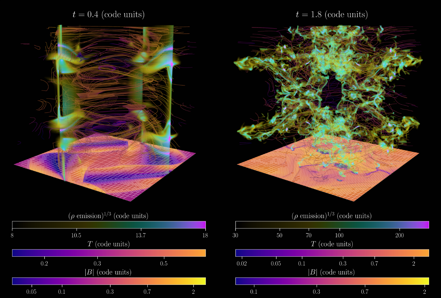
The run uses 4 AMR levels on a 100^3 base grid (effective 800^3), refined on density and energy, evolved to t=1.8. The evolution first shows the expected formation of current sheets and fast-mode shocks from compressive deformation of the magnetic "islands" (matching the known 2D case at t=0.4); by t=1.8 the initial slab symmetry is lost, and radiative cooling drives runaway condensation via thermal instability -- the same mechanism as the FFHD case above -- producing thin, connected, low-temperature sheets with density condensations in their folds. The paper's Figure 19 was rendered directly from the native .dat AMR snapshot using the Intel Embree ray-tracing library.

This case is a science demonstration (see the job_lumi_gpu_4l*.sh batch scripts for the full production run) and is not part of the automated make mhd regression suite; tests/mhd/Orszag-Tang_3D is instead the classic, non-cooled 3D Orszag-Tang verification test used there.

Special-relativistic hydrodynamics (tests/srhd/)

Relativistic jet -- jet_3D

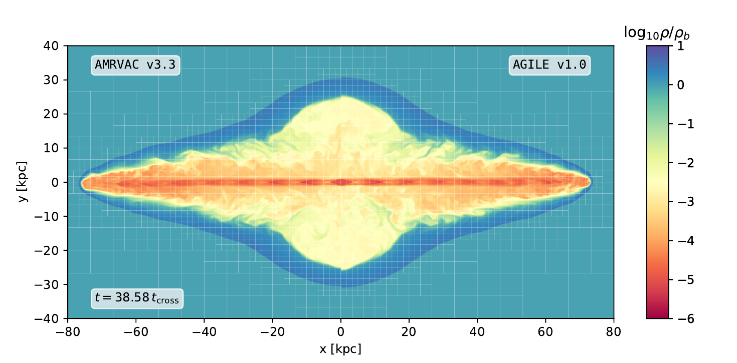
(paper Section 4.6) A relativistic jet propagation simulation demonstrating AGILE's special-relativistic hydrodynamics (SRHD) module, following the setup of Seo et al. (2021) (with reflective rather than outflow boundaries outside the jet nozzle, and the approximate Synge equation of state). An underdense jet (η = ρ_jet/ρ_ambient = 10^-5) is injected with Lorentz factor Γ = 7 into a uniform ambient medium representative of the hot intracluster medium (number density n = 10^-3 cm^-3, temperature 5×10^7 K). The jet inlet radius rj = 1000 pc sets a jet power of 1.09×10^45 erg/s (FR-II-like); the jet is resolved by 12 cells per rj, in a cubic domain of side 80 rj, and simulated for 6.5 Myr (42.8 jet-crossing times). AMR (4 levels) refines automatically on density gradients as the jet advances, growing from 300 blocks initially to 31296 by the end. Lax-Friedrichs fluxes, van Leer reconstruction, three-step Runge-Kutta time integration and CFL = 0.4 are used; no flooring or other robustness fallback is required.

As validation, the paper reruns the identical setup in MPI-AMRVAC (initial conditions and diagnostics are nearly 1:1 portable between the two codes) and finds very good qualitative agreement in jet morphology and recollimation-shock spacing (Figure 20). AGILE completed the run on one Snellius node (4×H100 GPUs) in 16 hours (3.02×10^8 CUPS/device, 1.2×10^9 CUPS total), 5.3 times faster -- and about 3.6 times cheaper in compute cost including IO -- than the equivalent MPI-AMRVAC run on 512 EPYC Rome CPU cores.